Adjusted Cost Base

In this vignette, we will demonstrate that calculations of the adjusted cost base by cryptoTax closely follows those of https://www.adjustedcostbase.ca/.

Basic ACB

To begin, we will replicate the basic ACB example showcased in https://www.adjustedcostbase.ca/blog/how-to-calculate-adjusted-cost-base-acb-and-capital-gains/

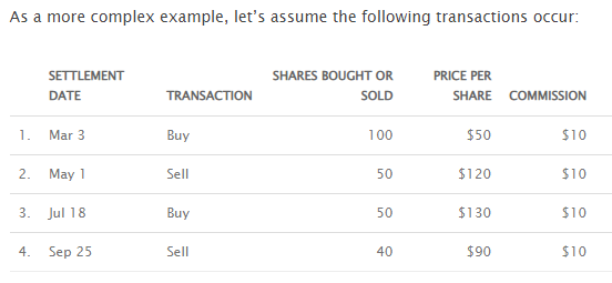
We first generate the data:

library(cryptoTax)
#> Error in get(paste0(generic, ".", class), envir = get_method_env()) : 
#>   object 'type_sum.accel' not found
data <- data_adjustedcostbase1
data

date	transaction	quantity	price	fees
2014-03-03	buy	100	50	10
2014-05-01	sell	50	120	10
2014-07-18	buy	50	130	10
2014-09-25	sell	40	90	10

Next, we generate the calculations to achieve the following result:

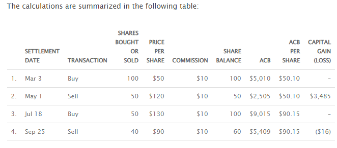
ACB(data, spot.rate = "price", sup.loss = FALSE)

date	transaction	quantity	price	fees	total.price	total.quantity	ACB	ACB.share	gains
2014-03-03	buy	100	50	10	5000	100	5010	50.10	NA
2014-05-01	sell	50	120	10	6000	50	2505	50.10	3485
2014-07-18	buy	50	130	10	6500	100	9015	90.15	NA
2014-09-25	sell	40	90	10	3600	60	5409	90.15	-16

Superficial losses

We will now replicate the more advanced superficial loss example showcased at https://www.adjustedcostbase.ca/blog/what-is-the-superficial-loss-rule/.

Example 1

We first demonstrate the “Violation of the Superficial Loss Rule” by using regular ACB without accounting for superficial losses:

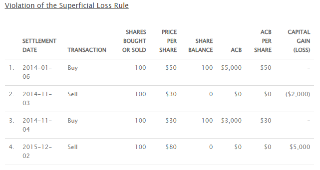
data <- data_adjustedcostbase2
ACB(data, spot.rate = "price", sup.loss = FALSE)

date	transaction	quantity	price	total.price	fees	total.quantity	ACB	ACB.share	gains
2014-01-06	buy	100	50	5000	0	100	5000	50	NA
2014-11-03	sell	100	30	3000	0	0	0	0	-2000
2014-11-04	buy	100	30	3000	0	100	3000	30	NA
2015-12-02	sell	100	80	8000	0	0	0	0	5000

Next, we do it the correct way, accounting for superficial losses:

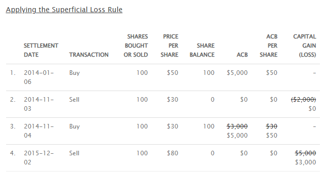
Per default, setting sup.loss = TRUE (the default) generates a lot of columns to provide as much information as possible. To make it look as short as the adjustedcostbase.ca example, we can subselect relevant columns:

library(dplyr)
ACB(data, spot.rate = "price") %>%
  select(date, transaction, quantity, price, total.quantity, ACB, ACB.share, gains)

date	transaction	quantity	price	total.quantity	ACB	ACB.share	gains
2014-01-06	buy	100	50	100	5000	50	NA
2014-11-03	sell	100	30	0	0	0	NA
2014-11-04	buy	100	30	100	5000	50	NA
2015-12-02	sell	100	80	0	0	0	3000

Example 2

We continue with the second superficial loss example. We first demonstrate the “Violation of the Superficial Loss Rule” by using regular ACB without accounting for superficial losses:

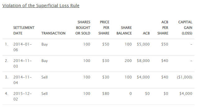
data <- data_adjustedcostbase3
ACB(data, spot.rate = "price", sup.loss = FALSE)

date	transaction	quantity	price	total.price	fees	total.quantity	ACB	ACB.share	gains
2014-01-06	buy	100	50	5000	0	100	5000	50	NA
2014-11-03	buy	100	30	3000	0	200	8000	40	NA
2014-11-04	sell	100	30	3000	0	100	4000	40	-1000
2015-12-02	sell	100	80	8000	0	0	0	0	4000

Next, we do it the correct way, accounting for superficial losses:

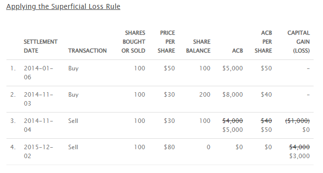
ACB(data, spot.rate = "price") %>%
  select(date, transaction, quantity, price, total.quantity, ACB, ACB.share, gains)

date	transaction	quantity	price	total.quantity	ACB	ACB.share	gains
2014-01-06	buy	100	50	100	5000	50	NA
2014-11-03	buy	100	30	200	8000	40	NA
2014-11-04	sell	100	30	100	5000	50	NA
2015-12-02	sell	100	80	0	0	0	3000

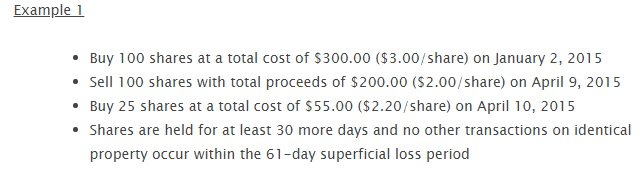
Example 3

We continue with the third superficial loss example (first example in https://www.adjustedcostbase.ca/blog/applying-the-superficial-loss-rule-for-a-partial-disposition-of-shares/). We first demonstrate the “Violation of the Superficial Loss Rule” by using regular ACB without accounting for superficial losses:

When Shares are Sold at a Loss and then Partially Reacquired within the Superficial Loss Period

data <- data_adjustedcostbase4
ACB(data, spot.rate = "price", sup.loss = FALSE)

date	transaction	quantity	price	total.price	fees	total.quantity	ACB	ACB.share	gains
2015-01-02	buy	100	3.0	300	0	100	300	3.0	NA
2015-04-09	sell	100	2.0	200	0	0	0	0.0	-100
2015-04-10	buy	25	2.2	55	0	25	55	2.2	NA

Next, we do it the correct way, accounting for superficial losses:

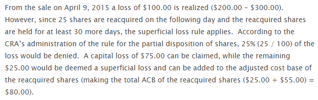
ACB(data, spot.rate = "price") %>%
  select(date, transaction, quantity, price, total.quantity, ACB, ACB.share, gains)

date	transaction	quantity	price	total.quantity	ACB	ACB.share	gains
2015-01-02	buy	100	3.0	100	300	3.0	NA
2015-04-09	sell	100	2.0	0	0	0.0	-75
2015-04-10	buy	25	2.2	25	80	3.2	NA

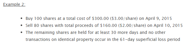
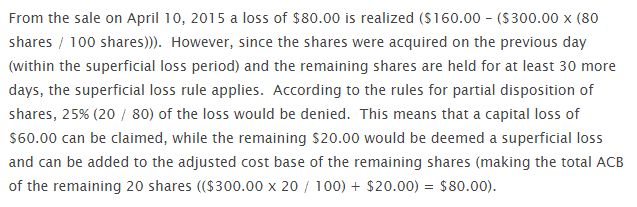
Example 4

We continue with the fourth superficial loss example (second example in https://www.adjustedcostbase.ca/blog/applying-the-superficial-loss-rule-for-a-partial-disposition-of-shares/). We first demonstrate the “Violation of the Superficial Loss Rule” by using regular ACB without accounting for superficial losses:

When Shares are Purchased and then Partially Sold within the Superficial Loss Period

data <- data_adjustedcostbase5
ACB(data, spot.rate = "price", sup.loss = FALSE)

date	transaction	quantity	price	total.price	fees	total.quantity	ACB	ACB.share	gains
2015-04-09	buy	100	3	300	0	100	300	3	NA
2015-04-10	sell	80	2	160	0	20	60	3	-80

Next, we do it the correct way, accounting for superficial losses:

ACB(data, spot.rate = "price") %>%
  select(date, transaction, quantity, price, total.quantity, ACB, ACB.share, gains)

date	transaction	quantity	price	total.quantity	ACB	ACB.share	gains
2015-04-09	buy	100	3	100	300	3	NA
2015-04-10	sell	80	2	20	80	4	NA

Example 5

When Multiple Acquisitions and/or Multiple Dispositions Occur Within the Superficial Loss Period

There are no examples given for this one, so we make our own. adjustedcostbase.ca writes that the web-based application does not support claiming partial losses automatically:

Note that AdjustedCostBase.ca does not automatically apply the superficial loss rule for you. Although you’ll see superficial loss rule warnings being displayed in many cases, it’s up to you to edit the transaction to apply the superficial loss rule. Also, in cases where you’re partially claiming a loss due to the superficial loss rule, you’ll need to manually calculate the partial capital loss using the methods described above.

Fortunately, cryptoTax allows claiming partial losses automatically. We first demonstrate the “Violation of the Superficial Loss Rule” by using regular ACB without accounting for superficial losses:

data <- data_adjustedcostbase6
ACB(data, spot.rate = "price", sup.loss = FALSE)

date	transaction	quantity	price	total.price	fees	total.quantity	ACB	ACB.share	gains
2015-04-09	buy	150	3	450	0	150	450	3	NA
2015-04-10	sell	20	2	40	0	130	390	3	-20
2015-04-15	buy	50	3	150	0	180	540	3	NA
2015-04-20	sell	10	2	20	0	170	510	3	-10
2015-05-15	sell	80	2	160	0	90	270	3	-80

Next, we do it the correct way, accounting for superficial losses, and include a few more columns for the demonstration:

ACB(data, spot.rate = "price") %>%
  select(
    date, transaction, quantity, price, total.quantity,
    suploss.range, sup.loss, sup.loss.quantity, ACB, ACB.share,
    gains.uncorrected, gains.sup, gains.excess, gains
  )

date	transaction	quantity	price	total.quantity	suploss.range	sup.loss	sup.loss.quantity	ACB	ACB.share	gains.uncorrected	gains.sup	gains.excess	gains
2015-04-09	buy	150	3	150	2015-03-10 UTC–2015-05-09 UTC	FALSE	0	450.0000	3.000000	0.00000	NA	NA	NA
2015-04-10	sell	20	2	130	2015-03-11 UTC–2015-05-10 UTC	TRUE	20	410.0000	3.153846	-20.00000	-20.00000	NA	NA
2015-04-15	buy	50	3	180	2015-03-16 UTC–2015-05-15 UTC	FALSE	0	580.0000	3.222222	0.00000	NA	NA	NA
2015-04-20	sell	10	2	170	2015-03-21 UTC–2015-05-20 UTC	TRUE	10	560.0000	3.294118	-12.22222	-12.22222	NA	NA
2015-05-15	sell	80	2	90	2015-04-15 UTC–2015-06-14 UTC	TRUE	80	361.1765	4.013072	-103.52941	-64.70588	-38.82353	-38.82353

Other examples from the internet

CryptoTaxCalculator

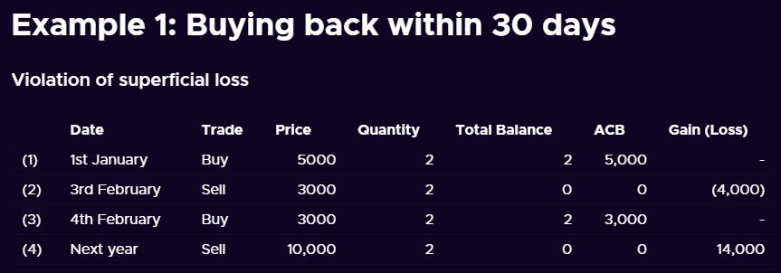
Example 1

Here is an example from CryptoTaxCalculator, showcased at: https://cryptotaxcalculator.io/guides/crypto-tax-canada-cra/. We first demonstrate the “Violation of the Superficial Loss Rule” by using regular ACB without accounting for superficial losses:

data <- data_cryptotaxcalculator1
ACB(data, transaction = "trade", spot.rate = "price", sup.loss = FALSE)

date	trade	currency	price	quantity	total.price	fees	total.quantity	ACB	ACB.share	gains
2020-01-01	buy	BTC	5000	2	10000	0	2	10000	5000	NA
2020-02-03	sell	BTC	3000	2	6000	0	0	0	0	-4000
2020-02-04	buy	BTC	3000	2	6000	0	2	6000	3000	NA
2021-02-04	sell	BTC	10000	2	20000	0	0	0	0	14000

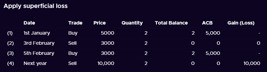
Next, we do it the correct way, accounting for superficial losses:

ACB(data, transaction = "trade", spot.rate = "price") %>%
  select(date, trade, price, quantity, total.quantity, ACB, ACB.share, gains)

date	trade	price	quantity	total.quantity	ACB	ACB.share	gains
2020-01-01	buy	5000	2	2	10000	5000	NA
2020-02-03	sell	3000	2	0	0	0	NA
2020-02-04	buy	3000	2	2	10000	5000	NA
2021-02-04	sell	10000	2	0	0	0	10000

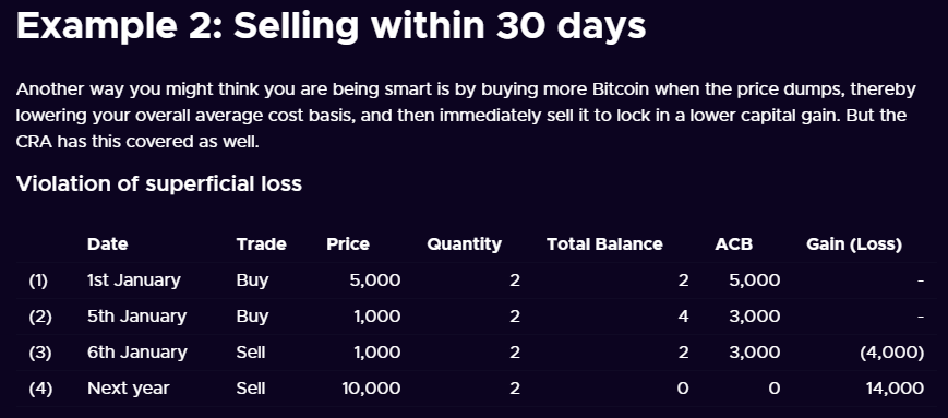
Example 2

We continue with the second superficial loss example. We first demonstrate the “Violation of the Superficial Loss Rule” by using regular ACB without accounting for superficial losses:

data <- data_cryptotaxcalculator2
ACB(data, transaction = "trade", spot.rate = "price", sup.loss = FALSE)

date	trade	currency	price	quantity	total.price	fees	total.quantity	ACB	ACB.share	gains
2020-01-01	buy	BTC	5000	2	10000	0	2	10000	5000	NA
2020-02-05	buy	BTC	1000	2	2000	0	4	12000	3000	NA
2020-02-06	sell	BTC	1000	2	2000	0	2	6000	3000	-4000
2021-02-06	sell	BTC	10000	2	20000	0	0	0	0	14000

Next, we do it the correct way, accounting for superficial losses:

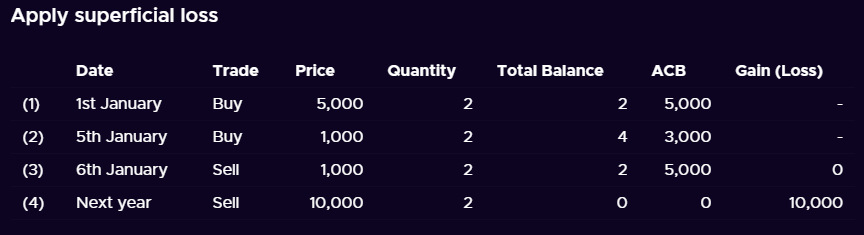
ACB(data, transaction = "trade", spot.rate = "price") %>%
  select(date, trade, price, quantity, total.quantity, ACB, ACB.share, gains)

date	trade	price	quantity	total.quantity	ACB	ACB.share	gains
2020-01-01	buy	5000	2	2	10000	5000	NA
2020-02-05	buy	1000	2	4	12000	3000	NA
2020-02-06	sell	1000	2	2	10000	5000	NA
2021-02-06	sell	10000	2	0	0	0	10000

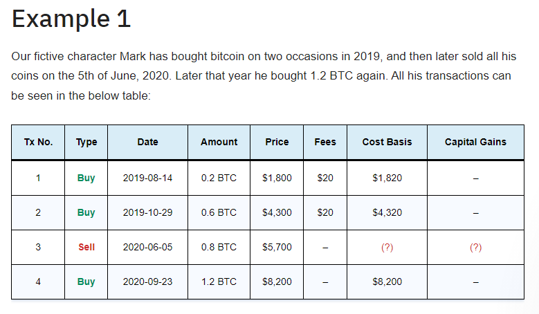
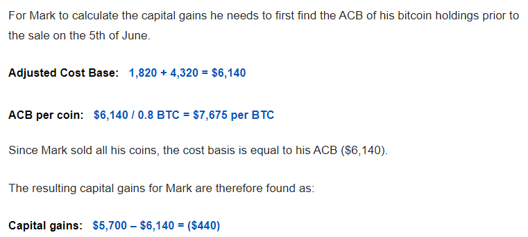
Coinpanda

Example 1

Here is an example from Coinpanda, showcased at: https://coinpanda.io/blog/crypto-taxes-canada-adjusted-cost-base/. The first example does not require the superficial loss rule so we can set it to FALSE without worry.

data <- data_coinpanda1
ACB(data,
  transaction = "type", quantity = "amount",
  total.price = "price", sup.loss = FALSE
)

type	date	currency	amount	price	fees	total.quantity	ACB	ACB.share	gains
buy	2019-08-14	BTC	0.2	1800	20	0.2	1820	9100.000	NA
buy	2019-10-29	BTC	0.6	4300	20	0.8	6140	7675.000	NA
sell	2020-06-05	BTC	0.8	5700	0	0.0	0	0.000	-440
buy	2020-09-23	BTC	1.2	8200	0	1.2	8200	6833.333	NA

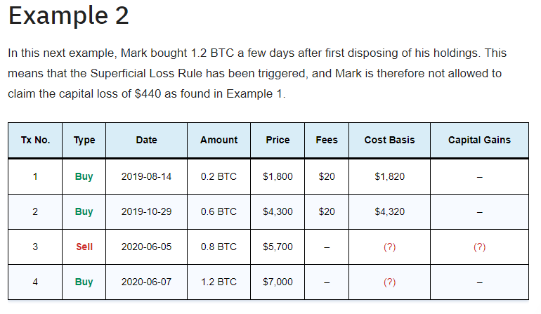
Example 2

We continue with the second superficial loss example. We first demonstrate the “Violation of the Superficial Loss Rule” by using regular ACB without accounting for superficial losses:

data <- data_coinpanda2
ACB(data,
  transaction = "type", quantity = "amount",
  total.price = "price", sup.loss = FALSE
)

type	date	currency	amount	price	fees	total.quantity	ACB	ACB.share	gains
buy	2019-08-14	BTC	0.2	1800	20	0.2	1820	9100.000	NA
buy	2019-10-29	BTC	0.6	4300	20	0.8	6140	7675.000	NA
sell	2020-06-05	BTC	0.8	5700	0	0.0	0	0.000	-440
buy	2020-06-07	BTC	1.2	7000	0	1.2	7000	5833.333	NA

Next, we do it the correct way, accounting for superficial losses:

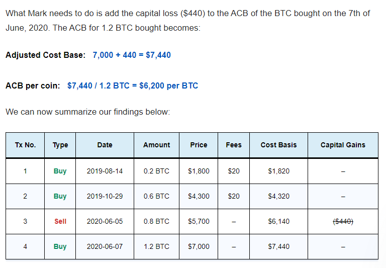
ACB(data, transaction = "type", quantity = "amount", total.price = "price") %>%
  select(type, date, amount, price, fees, ACB, ACB.share, gains)

type	date	amount	price	fees	ACB	ACB.share	gains
buy	2019-08-14	0.2	1800	20	1820	9100	NA
buy	2019-10-29	0.6	4300	20	6140	7675	NA
sell	2020-06-05	0.8	5700	0	0	0	NA
buy	2020-06-07	1.2	7000	0	7440	6200	NA

Koinly

Here is an example from Koinly, showcased at: https://koinly.io/blog/calculating-crypto-taxes-canada/. We first demonstrate the “Violation of the Superficial Loss Rule” by using regular ACB without accounting for superficial losses:

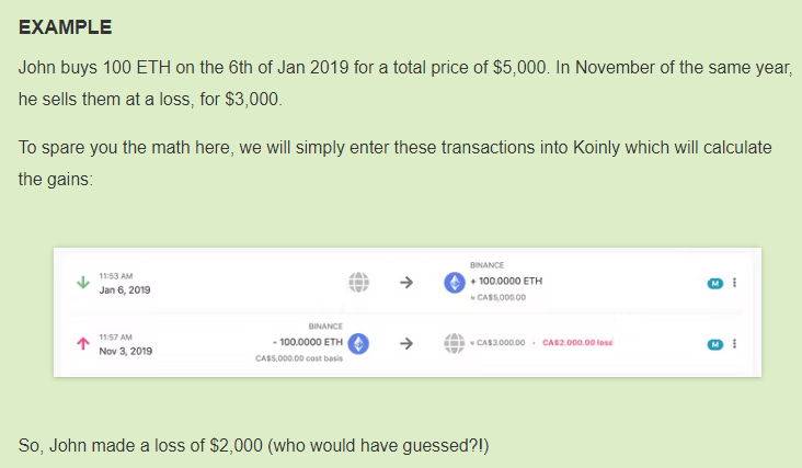
data <- data_koinly
ACB(data, sup.loss = FALSE)

date	transaction	currency	quantity	spot.rate	total.price	fees	total.quantity	ACB	ACB.share	gains
2019-01-06	buy	ETH	100	50	5000	0	100	5000	50	NA
2019-11-03	sell	ETH	100	30	3000	0	0	0	0	-2000
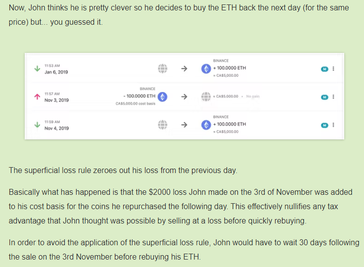
2019-11-04	buy	ETH	100	30	3000	0	100	3000	30	NA

Next, we do it the correct way, accounting for superficial losses:

ACB(data) %>%
  select(date, transaction, quantity, spot.rate, total.quantity, ACB, ACB.share, gains)

date	transaction	quantity	spot.rate	total.quantity	ACB	ACB.share	gains
2019-01-06	buy	100	50	100	5000	50	NA
2019-11-03	sell	100	30	0	0	0	NA
2019-11-04	buy	100	30	100	5000	50	NA